hicAggregateContacts

Background

hicAggregateContacts is a tool that allows plotting of aggregated Hi-C sub-matrices of a specified list of positions. Positions of interest can for example be binding sites of a specific protein that were determined by ChIP-seq or genetic elements as transcription start sites of active genes.

Description

Takes a list of positions in the Hi-C matrix and makes a pooled image.

usage: hicAggregateContacts --matrix MATRIX --outFileName OUTFILENAME --BED
                            BED --mode {inter-chr,intra-chr,all}
                            [--range RANGE] [--row_wise] [--BED2 BED2]
                            [--numberOfBins NUMBEROFBINS]
                            [--transform {total-counts,z-score,obs/exp,none}]
                            [--operationType {sum,mean,median}] [--perChr]
                            [--considerStrandDirection]
                            [--largeRegionsOperation {first,last,center}]
                            [--help] [--version]
                            [--outFilePrefixMatrix OUTFILEPREFIXMATRIX]
                            [--outFileContactPairs OUTFILECONTACTPAIRS]
                            [--outFileObsExp OUTFILEOBSEXP]
                            [--diagnosticHeatmapFile DIAGNOSTICHEATMAPFILE]
                            [--kmeans KMEANS] [--hclust HCLUST]
                            [--spectral SPECTRAL]
                            [--howToCluster {full,center,diagonal}]
                            [--keep_outlier] [--max_deviation MAX_DEVIATION]
                            [--chromosomes CHROMOSOMES [CHROMOSOMES ...]]
                            [--colorMap COLORMAP] [--plotType {2d,3d}]
                            [--vMin VMIN] [--vMax VMAX] [--dpi DPI]

Required arguments

--matrix, -m

Path of the Hi-C matrix to plot.

--outFileName, -out

File name to save the image.

--BED

Interactions between regions in this BED file are plotted.

--mode

Possible choices: inter-chr, intra-chr, all

Optional arguments

--range

Range of contacts that will be considered for plotting the aggregate contacts in bp with the format low_range:high_range for example 1000000:20000000. The range should start at contacts larger than TAD size to reduce background interactions. This will be ignored if inter-chromosomal contacts are of interest.

--row_wise

If given,the insteractions between each row of the BED file and its corresponding row of the BED2 file are computed. If intra-chromosomal contacts are computed, the rows with different chromosomes are ignored. If inter-chromosomal, the rows with same chromosomes are ignored. It keeps all the rows if all.

Default: False

--BED2

Optional second BED file. Interactions between regions in first and second BED file are plotted.

--numberOfBins

Number of bins to include in the submatrix. The bed regions will be centered between half number of bins and the other half number of bins (Default: 51).

Default: 51

--transform

Possible choices: total-counts, z-score, obs/exp, none

Type of transformation for the matrix. The options are “none”, “total-counts”, “z-score” and “obs/exp”. If total counts are selected, the sub-matrix values are divided by the total counts for normalization. If z-score or obs/exp are selected, the Hi-C matrix is converted into a z-score or observed / expected matrix (Default: “none”).

Default: “none”

--operationType

Possible choices: sum, mean, median

Type of the operation to be applied to summerize the submatrices into a single matrix. Options are sum, mean and median. (Default: “median”)

Default: “median”

--perChr

if set, it generates a plot per chromosome. It is only affected if intra-chromosomal contacts are of interest.

Default: False

--considerStrandDirection

This parameter specifies if the strand information is taken into account for the aggregation. It has the effect that the contacts of a reverse strand region are inverted e.g. [1,2,3] becomes [3,2,1].

Default: False

--largeRegionsOperation

Possible choices: first, last, center

If a given coordinate in the bed file is larger than a bin of the input matrix, by default only the first bin is taken into account. However there are more possibilities to handel such a case. Users can ask for the last bin or for center of the region. As an example if a region falls into bins [4,5,6] and –numberOfBins = 2 then if first, bins [3,4,5] are kept. If last: [5,6,7] and if center: [4,5,6].

Default: “first”

--version

show program’s version number and exit

--dpi

Optional parameter: Resolution for the image in case theoutput is a raster graphics image (e.g png, jpg) (Default: 300).

Default: 300

Output options

--outFilePrefixMatrix

If this option is set, the values underlying the output matrix will be saved to tab-delimited tables (one per chromosome) using the indicated prefix, for example TSS_to_TSS_chrX.tab. If clustering is performed, the values are saved including the cluster_id in the file TSS_to_TSS_chrX_cluster_1.tab.

--outFileContactPairs

Output file prefix. If this option is set, the position of the contact positions are saved as (chrom1, start1, end1, chrom2, start2, end2) where chrom_n, start_n, end_n correspond to the pair of positions used to compute the submatrix. The data is saved per chromosome and per cluster separately (one file each). The format is {prefix}_{chrom}_{cluster_id}.tab. If no clusters were computed, then only one file per chromosome is produced.

--outFileObsExp

writes the obs/exp matrix to a file, if –transform=obs/exp.

--diagnosticHeatmapFile

If given, a heatmap (per chromosome) is saved. Each row in the heatmap contains thediagonal of each of the submatrices centered on the bed file. This file is useful to get an idea of the values that are used for the aggregate matrix and to determine the fraction of sub-matrices that are aggregated that may have an enrichment at the center.

Clustering options

--kmeans

Number of clusters to compute. When this option is set, the submatrices are split into clusters (per chromosome) using the k-means algorithm.

--hclust

Number of clusters to compute (per chromosome). When this option is set, the matrix is split into clusters using the hierarchical clustering algorithm, using “ward linkage”. –hclust could be very slow if you have >1000 submatrices per chromosome. In those cases, you might prefer –kmeans

--spectral

Number of clusters to compute (per chromosome). When this option is set, the matrix is split into clusters using the spectral clustering algorithm.

--howToCluster

Possible choices: full, center, diagonal

Options are “full”, “center” and “diagonal”. The full clustering takes all values of each submatrix for clustering. “center”, takes only a square of length 3x3 from each submatrix and uses only this values for clustering. With the “diagonal” option the clustering is only carried out based on the submatrix diagonal (representing values at the same distance to each other) (Default: “full”).

Default: “full”

--keep_outlier

keep outliers before clustering. They will be removed by default. Note that removing outliers is also applied to the case where the number of clusters is one (e.g. no clustering is required) unless keep_outlier is set.

Default: False

--max_deviation

max deviation from mean to be determined as outlier.

Default: 2

Plotting options

--chromosomes, -C

List of chromosomes to plot.

--colorMap

Color map to use for the heatmap. Available values can be seen here: http://matplotlib.org/examples/color/colormaps_reference.html (Default: “RdYlBu_r”).

Default: “RdYlBu_r”

--plotType

Possible choices: 2d, 3d

Plot type (Default: “2d”).

Default: “2d”

--vMin

Minimum value of the plotted score.

--vMax

Maximum value of the plotted score.

Usage example

Below, you can find an example of an aggregate Hi-C matrix obtained from Drosophila melanogaster Hi-C data. The interactions are plotted at binding sites of a protein that were determined by ChIP-seq. We plot sub-matrices of 30 bins (1.5 kb bin size, 45 kb in total). The regions specified in the BED file will be centered between half number of bins and the other half number of bins.The considered range is 300-1000 kb. The range should be adjusted and only contain contacts larger than TAD size to reduce background interactions.

$ hicAggregateContacts --matrix Dmel.h5 --BED ChIP-seq-peaks.bed \
--outFileName Dmel_aggregate_Contacts --vMin 0.8 --vMax 2.2 \
--range 300000:1000000 --numberOfBins 30 --chromosomes X \
--operationType mean --transform obs/exp --mode intra-chr

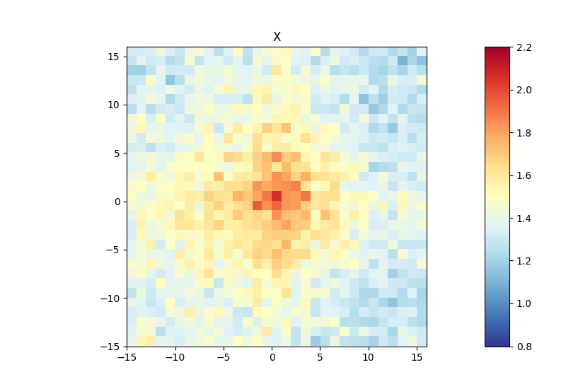
This example was calculated using mean interactions of an observed vs expected transformed Hi-C matrix. Additional options for the matrix transformation are total-counts or z-score. Aggregate contacts can be plotted in 2D or 3D.