Example usage
How we use HiCExplorer
To generate a Hi-C contact matrix is necessary to perform the following basic steps
Map the Hi-C reads to the reference genome
Filter the aligned reads to create a contact matrix
Filter matrix bins with low or zero read coverage
Remove biases from the Hi-C contact matrices
After a corrected Hi-C matrix is created other tools can be used to visualize it, call TADS or compare it with other matrices.
Reads mapping
Mates have to be mapped individually to avoid mapper specific heuristics designed for standard paired-end libraries.
We have used the HiCExplorer successfully with bwa, bowtie2 and hisat2. However, it is important to:
for either bowtie2`or `hisat2 use the –reorder parameter which tells bowtie2 or hisat2 to output the sam files in the exact same order as in the .fastq files.
use local mapping, in contrast to end-to-end. A fraction of Hi-C reads are chimeric and will not map end-to-end thus, local mapping is important to increase the number of mapped reads.
Tune the aligner parameters to penalize deletions and insertions. This is important to avoid aligned reads with gaps if they happen to be chimeric.
# map the reads, each mate individually using
# for example bwa
#
# bwa mem mapping options:
#       -A INT        score for a sequence match, which scales options -TdBOELU unless overridden [1]
#       -B INT        penalty for a mismatch [4]
#       -O INT[,INT]  gap open penalties for deletions and insertions [6,6]
#       -E INT[,INT]  gap extension penalty; a gap of size k cost '{-O} + {-E}*k' [1,1] # this is set very high to avoid gaps
#                                  at restriction sites. Setting the gap extension penalty high, produces better results as
#                                  the sequences left and right of a restriction site are mapped independently.
#       -L INT[,INT]  penalty for 5'- and 3'-end clipping [5,5] # this is set to no penalty.

$ bwa mem -A1 -B4  -E50 -L0  index_path \
    mate_R1.fastq.gz 2>>mate_R1.log | samtools view -Shb - > mate_R1.bam

$ bwa mem -A1 -B4  -E50 -L0  index_path \
    mate_R2.fastq.gz 2>>mate_R2.log | samtools view -Shb - > mate_R2.bam
Creation of a Hi-C matrix
Once the reads have been mapped the Hi-C matrix can be built. For this, the minimal extra information required is the binSize used for the matrix. Is it best to enter a low number like 10.000 because lower resolution matrices (larger bins) can be easily constructed using hicMergeMatrixBins. Matrices at restriction fragment resolution can be created by providing a file containing the restriction sites, this file can be created with the tool hicFindRestSites
hicFindRestSites that is part of HiCExplorer.
# build matrix from independently mated read pairs
# the restriction sequence GATC is recognized by the DpnII restriction enzyme

$ hicBuildMatrix --samFiles mate_R1.bam mate_R2.bam \
                 --binSize 10000 \
                 --restrictionSequence GATC \
                 --danglingSequence GATC \
                 --restrictionCutFile cut_sites.bed \
                 --threads 4 \
                 --inputBufferSize 100000 \
                 --outBam hic.bam \
                 -o hic_matrix.h5 \
                 --QCfolder ./hicQC
hicBuildMatrix creates two files, a bam file containing only the valid Hi-C read pairs and a matrix containing the Hi-C contacts at the given resolution. The bam file is useful to check the quality of the Hi-C library on the genome browser. A good Hi-C library should contain piles of reads near the restriction fragment sites. In the QCfolder a html file is saved with plots containing useful information for the quality control of the Hi-C sample like the number of valid pairs, duplicated pairs, self-ligations etc. Usually, only 25%-40% of the reads are valid and used to build the Hi-C matrix mostly because of the reads that are on repetitive regions that need to be discarded.
An important quality control measurement to check is the inter chromosomal fraction of reads as this is an indirect measure of random Hi-C contacts. Good Hi-C libraries have lower than 10% inter chromosomal contacts. The hicQC module can be used to compare the QC measures from different samples.
Correction of Hi-C matrix
The Hi-C matrix has to be corrected to remove GC, open chromatin biases and, most importantly, to normalize the number of restriction sites per bin. Because a fraction of bins from repetitive regions contain few contacts it is necessary to filter those regions first. Also, in mammalian genomes some regions enriched by reads should be discarded. To aid in the filtering of regions hicCorrectMatrix generates a diagnostic plot as follows:
$ hicCorrectMatrix diagnostic_plot -m hic_matrix.h5 -o hic_corrected.png
The plot should look like this:
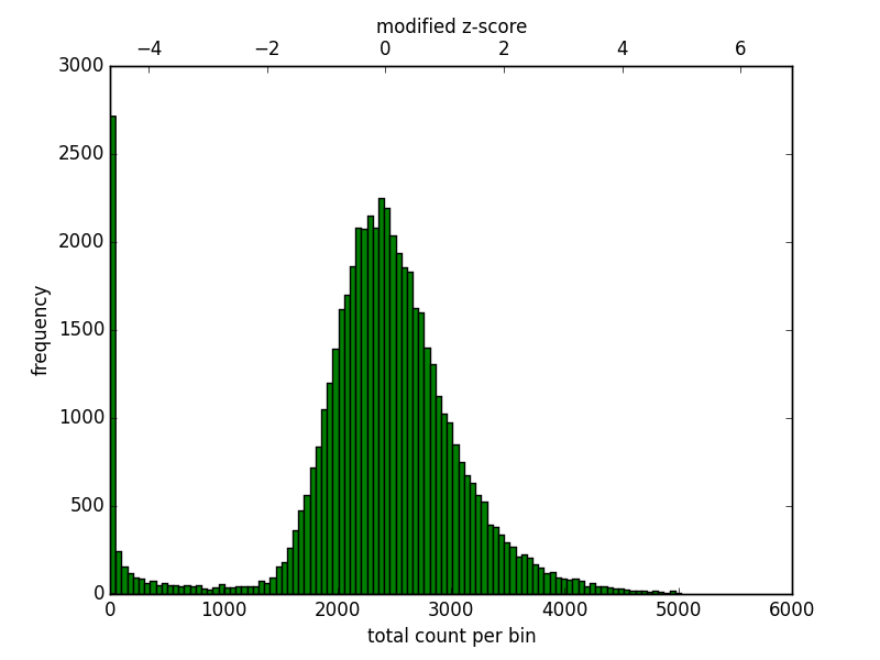
Histogram of the number of counts per bin.
For the upper threshold is only important to remove very high outliers and thus a value of 5 could be used. For the lower threshold it is recommended to use a value between -2 and -1. What it not desired is to try to correct low count bins which could result simply in an amplification of noise. For the upper threshold is not so concerning because those bins will be scaled down.
Once the thresholds have been decided, the matrix can be corrected
# correct Hi-C matrix
$ hicCorrectMatrix correct -m hic_matrix.h5 --filterThreshold -1.5 5 -o hic_corrected.h5
In the case of multiple samples / replicates that need to be normalized to the same read coverage we recommend to compute first the normalization (with hicNormalize) and correct the data (with hicCorrectMatrix) in a second step.
Visualization of results
There are two ways to see the resulting matrix, one using hicPlotMatrix and the other is using hicPlotTADs. The first one allows the visualization over large regions while the second one is preferred to see specific parts together with other information, for example genes or bigwig tracks.
Because of the large differences in counts found int he matrix, it is better to plot the counts using the –log1p option.
$ hicPlotMatrix -m hic_corrected.h5 -o hic_plot.png --region 1:20000000-80000000 --log1p
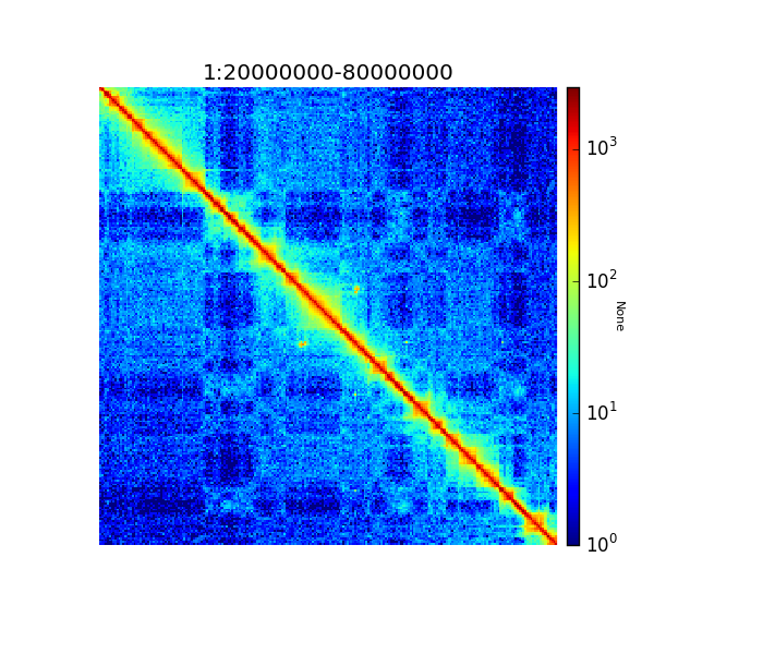
Corrected Hi-C counts in log scale.
Quality control of Hi-C data and biological replicates comparison
HiCExplorer integrates multiple tools that allow the evaluation of the quality of Hi-C libraries and matrices.
hicQC on the log files produced by hicBuildMatrix and control of the pdf file produced.
Proportion of useful reads is important to assess the efficiency of the HiC protocol, which is dependant of proportion of dangling ends detected… Proportion of inter chromosomal, short range and long range contacts are important for….
hicPlotDistVsCounts to compare the distribution of corrected Hi-C counts in relation with the genomic
distance between multiple samples. If some differences are observed between biological replicates, these can be investigated more precisely by computing log2ratio matrices.
hicCompareMatrices log2ratio of matrices of biological replicates to identify where the potential changes are located.
hicPlotPCA bins correlation of two biological replicates.
TAD calling
To call TADs a corrected matrix is needed. Restriction fragment resolution matrices provide the best results. TAD calling works in two steps: First HiCExplorer computes a TAD-separation score based on a z-score matrix for all bins. Then those bins having a local minimum of the TAD-separation score are evaluated with respect to the surrounding bins to decide assign a p-value. Then a cutoff is applied to select the bins more likely to be TAD boundaries.
$ hicFindTADs -m hic_corrected.h5 --outPrefix hic_corrected --numberOfProcessors 16
This code will produce several files: 1. The TAD-separation score file, 2. the z-score matrix, 3. a bed file with the boundary location, 4. a bed file with the domains, 5. a bedgraph file with the TAD-score that can be visualized in a genome browser.
The TAD-separation score and the matrix can be visualized using hicPlotTADs.
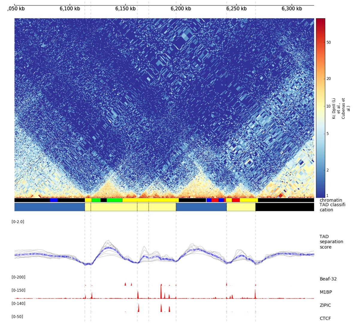
Example output from hicPlotTADs from http://chorogenome.ie-freiburg.mpg.de/
A / B compartment analysis
To compute the A / B compartments the matrix needs to be transformed to an observed/expected matrix in the way Lieberman-Aiden describes it. In a next step a pearson correlation matrix and based on it a covariance matrix is computed. Finally the eigenvectors based on the covariance matrix are computed. All these steps are computed with the command:
$ hicPCA -m hic_corrected.h5 --outFileName pca1.bw pca2.bw --format bigwig
If the intermediate matrices of this process should be used for plotting run:
$ hicTransform -m hic_corrected.h5 --outFileName all.h5 --method all
This creates all intermediate matrices: obs_exp_all.h5, pearson_all.h5 and covariance_all.h5.
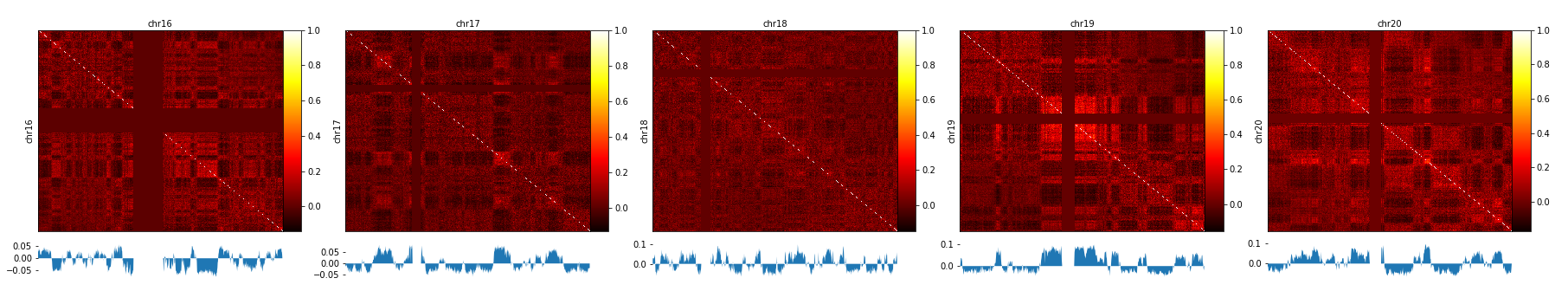
The A / B compartments can be plotted with hicPlotMatrix.
$ hicPlotMatrix -m pearson_all.h5 --outFileName pca1.png --perChr --bigwig pca1.bw