Captured Hi-C data analysis
How we use HiCExplorer to analyse cHi-C data
This How-to is based on the published dataset from Andrey et al. 2017. For the tutorial, we use the samples FL-E13.5 and MB-E-10.5.
Disclaimer: With HiCExplorer 3.7 all data is stored in hdf5 based files to make the handling easier. Please check your version of HiCExplorer to make sure you use the latest version. Commands of older HiCExplorer version do not work with the introduced changes!
Download the raw data
Please download the raw data via the following links or via NCBI GSE84795 .
Dataset |
forward |
reverse |
|---|---|---|
CC-FL-E135-Wt-Mm-Rep1 |
||
CC-FL-E135-Wt-Mm-Rep2 |
||
CC-MB-E105-Wt-Mm-Rep1 |
||
CC-MB-E105-Wt-Mm-Rep2 |
Mapping
Map the files with a mapper of your choice against the mm9 reference genome; as an example, the mapping with bowtie2 is shown.
bowtie2 -x mm9_index --threads 8 -U SRR3950565_1.fastq.gz --reorder | samtools view -Shb - > SRR3950565_1.bam
bowtie2 -x mm9_index --threads 8 -U SRR3950565_2.fastq.gz --reorder | samtools view -Shb - > SRR3950565_2.bam
bowtie2 -x mm9_index --threads 8 -U SRR3950566_1.fastq.gz --reorder | samtools view -Shb - > SRR3950566_1.bam
bowtie2 -x mm9_index --threads 8 -U SRR3950566_2.fastq.gz --reorder | samtools view -Shb - > SRR3950566_2.bam
bowtie2 -x mm9_index --threads 8 -U SRR3950559_1.fastq.gz --reorder | samtools view -Shb - > SRR3950559_1.bam
bowtie2 -x mm9_index --threads 8 -U SRR3950559_2.fastq.gz --reorder | samtools view -Shb - > SRR3950559_2.bam
bowtie2 -x mm9_index --threads 8 -U SRR3950560_1.fastq.gz --reorder | samtools view -Shb - > SRR3950560_1.bam
bowtie2 -x mm9_index --threads 8 -U SRR3950560_2.fastq.gz --reorder | samtools view -Shb - > SRR3950560_2.bam
Create cHi-C matrices
To create a cHi-C matrix we use HiCExplorer’s hicBuildMatrix for each replicate separately and merge the replicates into a single matrix later. Like Andrey et al., we use a resolution of 1kb and use the restriction enzyme DpnII.
hicBuildMatrix --samFiles SRR3950565_1.bam SRR3950565_2.bam  --binSize 1000 --restrictionSequence GATC --outFileName SRR3950565.cool --QCfolder SRR3950565_QC --threads 6
hicBuildMatrix --samFiles SRR3950566_1.bam SRR3950566_2.bam  --binSize 1000 --restrictionSequence GATC --outFileName SRR3950566.cool --QCfolder SRR3950566_QC --threads 6
hicBuildMatrix --samFiles SRR3950559_1.bam SRR3950559_2.bam  --binSize 1000 --restrictionSequence GATC --outFileName SRR3950559.cool --QCfolder SRR3950559_QC --threads 6
hicBuildMatrix --samFiles SRR3950560_1.bam SRR3950560_2.bam  --binSize 1000 --restrictionSequence GATC --outFileName SRR3950560.cool --QCfolder SRR3950560_QC --threads 6
hicSumMatrix --matrices SRR3950565.cool SRR3950566.cool --outFileName FL-E13-5.cool
hicSumMatrix --matrices SRR3950559.cool SRR3950560.cool --outFileName MB-E10-5.cool
Terminology: Reference point vs viewpoint
A reference point is one single genomic position i.e. chr1 500 510 is a reference point. A viewpoint is in contrast the region defined by the reference point and the up and downstream range, i.e. range 100 and reference point chr1 50 70 leads to the viewpoint chr1 400 610.
Creation of reference point file
Andrey et al. state that they used a total of 460 reference points, but that 24 were removed due to low sequence coverage or non-correspondence to a promoter region, leading to 446 in total.
To reproduce this, we need all reference points which are published in Supplementary Table S2 and S8.
It is simplest to create the reference point file in the following format using Excel and store it as a tab separated file:
chr1 4487435 4487435 Sox17
Otherwise, just download the prepared file. We will do the quality control on our own and compare with the results of Andrey et al.
Quality control
As a first step we compute the quality of each viewpoint by considering the sparsity. As soon as one viewpoint in one sample is less than the user-defined threshold (–sparsity), the reference point is no longer considered.
chicQualityControl -m FL-E13-5.cool MB-E10-5.cool -rp reference_points.bed --sparsity 0.025 --threads 20
The quality control creates five files: two plots showing the sparsity structure of the samples and three files containing the accepted reference points, the rejected ones and one file with all viewpoints and their sparsity level per sample.
In our example the plots look like the following:
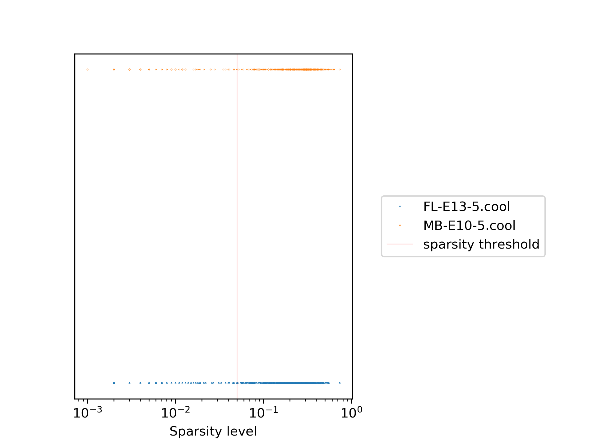
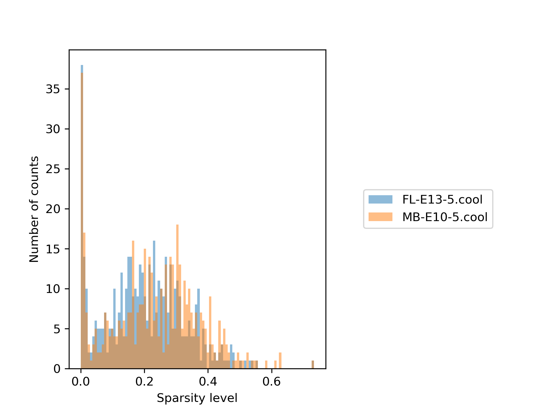
The first plot shows the sparsity per sample for each viewpoint, while the second one shows the sparsity distribution as a histogram. It can be seen quite clearly that only a minority of the samples are really sparse and therefore need to be removed. The red line indicates the chosen sparsity level.
The reference point Tdap2b at chr1 19198995, which has a sparsity of 0.018 in FL-E13-5 and 0.016 in MB-E10-5, is considered to be of bad quality. To confirm this result we plot the viewpoint:
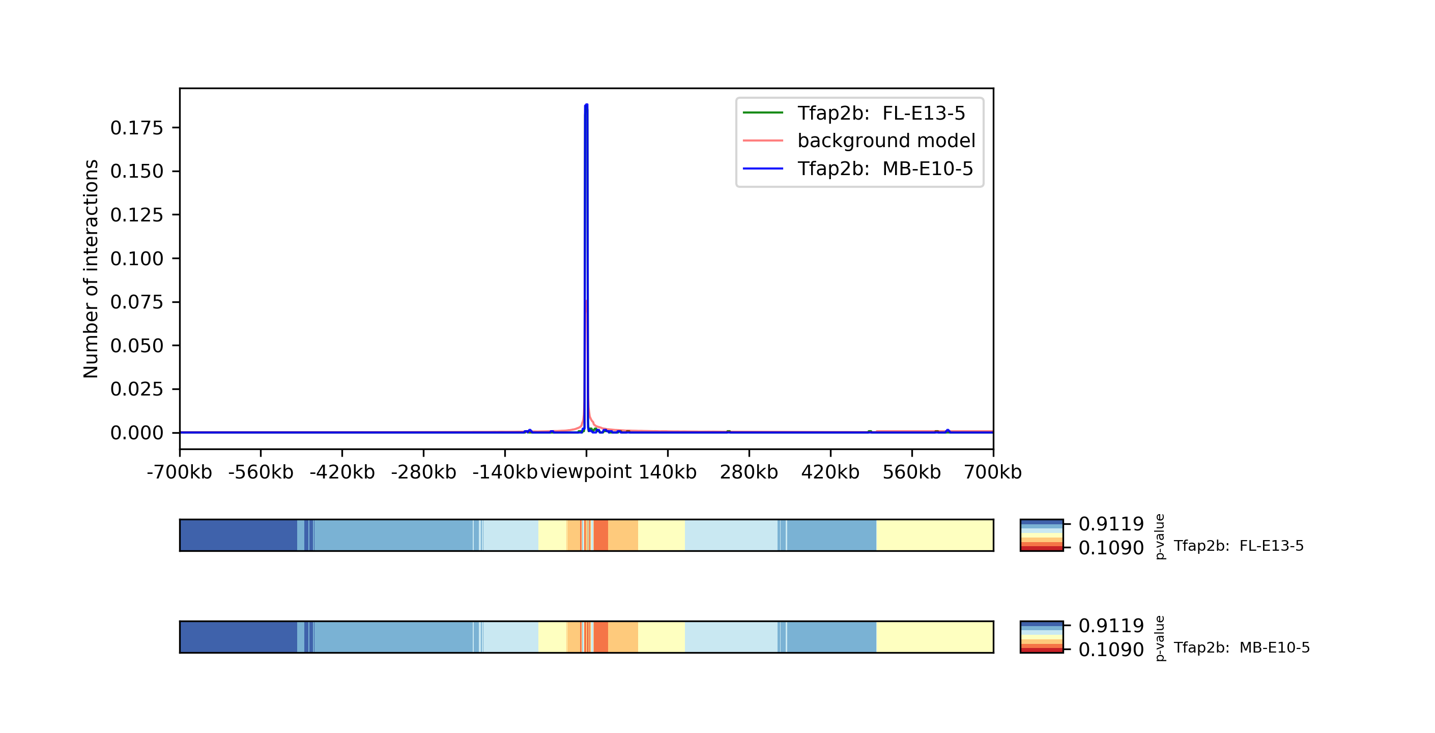
The plot shows there are effectively no interactions except with the reference point itself and confirm the point should be removed from the data.
The result of the quality control rejected 71 reference points as too sparse, but surprisingly the viewpoints rejected by Andrey et al. are accepted. An explanation for this could be that we only consider two samples and not all samples used by Andrey, and therefore we missed the bad quality of some viewpoints.
Please consider that this bad viewpoint was selected arbitrary out of the sample data and is only an example.
Download the data: Filtered reference points, Quality control raw data and rejected reference points.
Background model
The background model computes all viewpoints given by the reference points for both samples in a range defined by the parameter fixateRange. We recommend setting it to 500kb because real interactions above the range are rarely observed and very low interaction numbers such as 1 are already considered to be significant. With this setting, only the interactions in a range 500kb up- and downstream of the reference point are considered for each viewpoint. Based on this data, two background models are computed; the first one computes the average per relative distance to the reference point, and secondly, a negative binomial distribution per relative distance to the reference point is fitted. This first model is used for filtering in the significant interaction evaluation by an x-fold factor and for plotting. The negative binomial model is more important; it is used to compute a p-value per relative distance in each sample, which is used to make the decision if an interaction is considered as significant.
chicViewpointBackgroundModel -m FL-E13-5.cool MB-E10-5.cool --fixateRange 500000 -t 20 -rp reference_points.bed -o background_model.txt
The background model looks like this:
Relative position   size nbinom     prob nbinom     max value       mean value
-500000             75.895607451213 0.998528939430  2.333333333333  0.000101543771
-499000             90.348171762247 0.998725799952  2.750000000000  0.000104681360
-498000             78.512621775755 0.998514111424  2.800000000000  0.000106107536
-497000             75.706478185610 0.998327784087  3.800000000000  0.000116147819
You can download the background model.
Viewpoint computation
In this step the viewpoints for each reference point listed in a reference_points.bed-file is extracted from the interaction matrix, using the quality controlled file created by chicQualityControl. The up- and downstream range can be given via –range upstream downstream. Please use the same value for –fixateRange as in the background model computation. For each relative distance the x-fold over the average value of this relative distance is computed and each location is assigned a p-value based on the background negative binomial distribution for this relative distance. The output is one hdf5 based file containing all the data.
chicViewpoint -m FL-E13-5.cool MB-E10-5.cool --averageContactBin 5 --range 1000000 1000000 -rp referencePoints.bed -bmf background_model.txt --outFileName interactions.hdf5 --fixateRange 500000 --threads 20
chicExportData --file interactions.hdf5 --outputMode all -o interactions.tar.gz -t 16
The text files for each matrix and viewpoint have the following structure:
# Chromosome        Start   End     Gene    Sum of interactions     Relative position       Relative Interactions   p-value x-fold  Raw
chr1        14167000        14168000        Eya1    673.000000000000        -133000 0.000000000000  1.000000000000  0.000000000000  0.000000000000
chr1        14168000        14169000        Eya1    673.000000000000        -132000 0.000000000000  1.000000000000  0.000000000000  0.000000000000
chr1        14169000        14170000        Eya1    673.000000000000        -131000 0.000000000000  1.000000000000  0.000000000000  0.000000000000
chr1        14170000        14171000        Eya1    673.000000000000        -130000 0.000000000000  1.000000000000  0.000000000000  0.000000000000
chr1        14171000        14172000        Eya1    673.000000000000        -129000 0.000000000000  1.000000000000  0.000000000000  0.000000000000
chr1        14172000        14173000        Eya1    673.000000000000        -128000 0.000000000000  1.000000000000  0.000000000000  0.000000000000
chr1        14173000        14174000        Eya1    673.000000000000        -127000 0.000000000000  1.000000000000  0.000000000000  0.000000000000
chr1        14174000        14175000        Eya1    673.000000000000        -126000 0.000000000000  1.000000000000  0.000000000000  0.000000000000
chr1        14175000        14176000        Eya1    673.000000000000        -125000 0.000297176820  0.042850447268  0.916568982282  0.200000000000
chr1        14176000        14177000        Eya1    673.000000000000        -124000 0.000297176820  0.042850447268  0.908160092485  0.200000000000
Each file contains a header with information about content of the different columns.
Significant interactions detection
To detect significant interactions and to prepare a target file for each viewpoint which will be used for the differential analysis, the script chicSignificantInteractions is used. It offers two modes: either the user can specify an x-fold value or a loose p-value. The first one considers all interactions with a minimum x-fold over the average background for its relative distribution as a candidate or secondly, all interactions with a loose p-value or less are considered. These are pre-selection steps to be able to detect wider peaks in the same way as sharp ones. All detected candidates are merged to one peak if they are direct neighbors, and the sum of all interaction values of this neighborhood is used to compute a new p-value. The p-value is computed based on the relative distance continuous negative binomial distribution of the interaction with the original highest interaction value. All peaks considered are accepted as significant interactions if their p-value is as small as the threshold –pvalue.
To exclude interactions with an interaction value smaller than desired the parameter –peakInteractionsThreshold can be set.
In this example we use the created interactions.hdf5 file of chicViewpoint, a loose p-value of 0.1 and p-value of 0.01. For all stored locations the significant interactions are computed:
chicSignificantInteractions --interactionFile interactions.hdf5 -bmf background_model.txt --range 1000000 1000000 --pValue 0.01 --loosePValue 0.1 --outFileNameSignificant significant.hdf5 --outFileNameTarget target.hdf5 --combinationMode dual
This creates two files, a file storing all significant interactions, significant.hdf5, and a target file, target.hdf5. The content of the two files can be export via chicExport:
chicExportData --file significant.hdf5 --outputMode all -o targets.tar.gz  -t 16
chicExportData --file target.hdf5 --outputMode all -o targets.tar.gz  -t 16
For all tools it is also possible to just extract one gene by the gene name as it was given in the fourth column of the reference file. For each name, the data for all stored matrices is extracted. This mode works also on the interactions, target, aggregated and differential files.
chicExportData --file significant.hdf5 --outputMode geneName --outputModeName Eya1 -t 16
The significant interaction files looks like the following:
# Chromosome        Start   End     Gene    Sum of interactions     Relative position       Relative Interactions   p-value x-fold  Raw
chr1        14274000        14278000        Eya1    673.000000000000        -26000  0.008320950966  0.007037698679  7.811125758170  5.600000000000
chr1        14296000        14298000        Eya1    673.000000000000        -3000   0.057949479941  0.104215728599  3.781355935916  39.000000000000
chr1        14314000        14316000        Eya1    673.000000000000        14000   0.015156017831  0.048507853154  3.190333935010  10.200000000000
chr1        14317000        14319000        Eya1    673.000000000000        17000   0.014561664190  0.034914431882  3.517090338584  9.800000000000
chr1        14480000        14488000        Eya1    673.000000000000        184000  0.011292719168  0.000000010481  19.285082946462 7.600000000000
chr1        14491000        14501000        Eya1    673.000000000000        200000  0.030683506686  0.000000000000  56.967824833429 20.650000000000
The target file looks like:
chr1        14274000        14278000
chr1        14295000        14298000
chr1        14314000        14319000
chr1        14426000        14432000
chr1        14447000        14455000
chr1        14460000        14465000
chr1        14480000        14488000
chr1        14491000        14501000
The parameter –combinationMode has the options single and dual. This parameter is important if a differential analysis should be computed, either a target region is only for one gene of one matrix, or the regions of one gene of two matrices are combined. For example: - dual combines as follows: [[matrix1_gene1, matrix2_gene1], [matrix2_gene1, matrix3_gene1],[matrix1_gene2, matrix2_gene2], …] - single combines as follows: [matrix1_gene1, matrix1_gene2, matrix2_gene1, …]
Aggregate data for differential test
The process to aggregate data is only necessary if the differential test is used. chicAggregateStatistic takes the created interaction file from chicViewpoint as input and either the target file created by chicSignificantInteractions or one target file which applies for all viewpoints.
chicAggregateStatistic --interactionFile interaction.hdf5 --targetFile target.hdf5 --outFileName aggregate.hdf5 -t 16
chicAggregateStatistic --interactionFile interaction.hdf5 --targetFile regions_of_interest.bed --outFileName aggregate.hdf5 -t 16
It selects the original data based on the target locations and returns one hdf5 based file.
Differential test
The differential test tests the interaction value of the reference point and the interaction value of the target of two samples for a differential expression. To achieve this, either Fisher’s test or the chi-squared test can be used. H0 is defined as ‘both locations are equal’, meaning the differential expressed targets can be found in the H0 rejected file.
chicDifferentialTest --aggregatedFile aggregate.hdf5 --alpha 0.05 --statisticTest fisher --outFileName differential.hdf5 -t 16
It is important to set the desired alpha value and the output is written to one hdf5 based file. For each sample three internal datasets are created:
H0 rejected targets
H0 accepted targets
one file containing both
The data can be exported via chicExportData:
chicExportData --file differential.hdf5 --outputMode all -o differential.tar.gz -t 16
The created tar.gz file contains for each tested regions the three files rejected, ‘accepted’ and a file containing both information. It is also possible to extract only one gene:
chicExportData --file differential.hdf5 --outputMode geneName --outputModeName Eya1 -o differential_one -t 16
In case of the single extraction, the output file name serves only to determine the folder to save the data. The names are based on the gene name.
# Chromosome        Start   End     Gene    Relative distance       sum of interactions 1   target_1 raw    sum of interactions 2   target_2 raw    p-value
chr1        14274000        14278000        Eya1    -23000  673.000000000000        5.600000000000  832.000000000000        0.000000000000  0.008134451704
chr1        14295000        14298000        Eya1    -3000   673.000000000000        44.400000000000 832.000000000000        49.800000000000 0.670801771179
chr1        14314000        14319000        Eya1    18000   673.000000000000        24.200000000000 832.000000000000        23.400000000000 0.385952554141
chr1        14426000        14432000        Eya1    131000  673.000000000000        2.400000000000  832.000000000000        9.000000000000  0.245228952263
chr1        14447000        14455000        Eya1    154000  673.000000000000        4.400000000000  832.000000000000        12.400000000000 0.232102031454
chr1        14460000        14465000        Eya1    164000  673.000000000000        3.200000000000  832.000000000000        7.600000000000  0.564250349826
chr1        14480000        14488000        Eya1    187000  673.000000000000        7.600000000000  832.000000000000        3.200000000000  0.151571165731
chr1        14491000        14501000        Eya1    200000  673.000000000000        20.650000000000 832.000000000000        18.750000000000 0.338670136491
Plotting of Viewpoints
chicPlotViewpoint can plot viewpoints of one gene in one plot, add the mean background, show the p-value per relative distance per sample as an additional heatmap bar and highlight significant interactions or differential expressed regions.
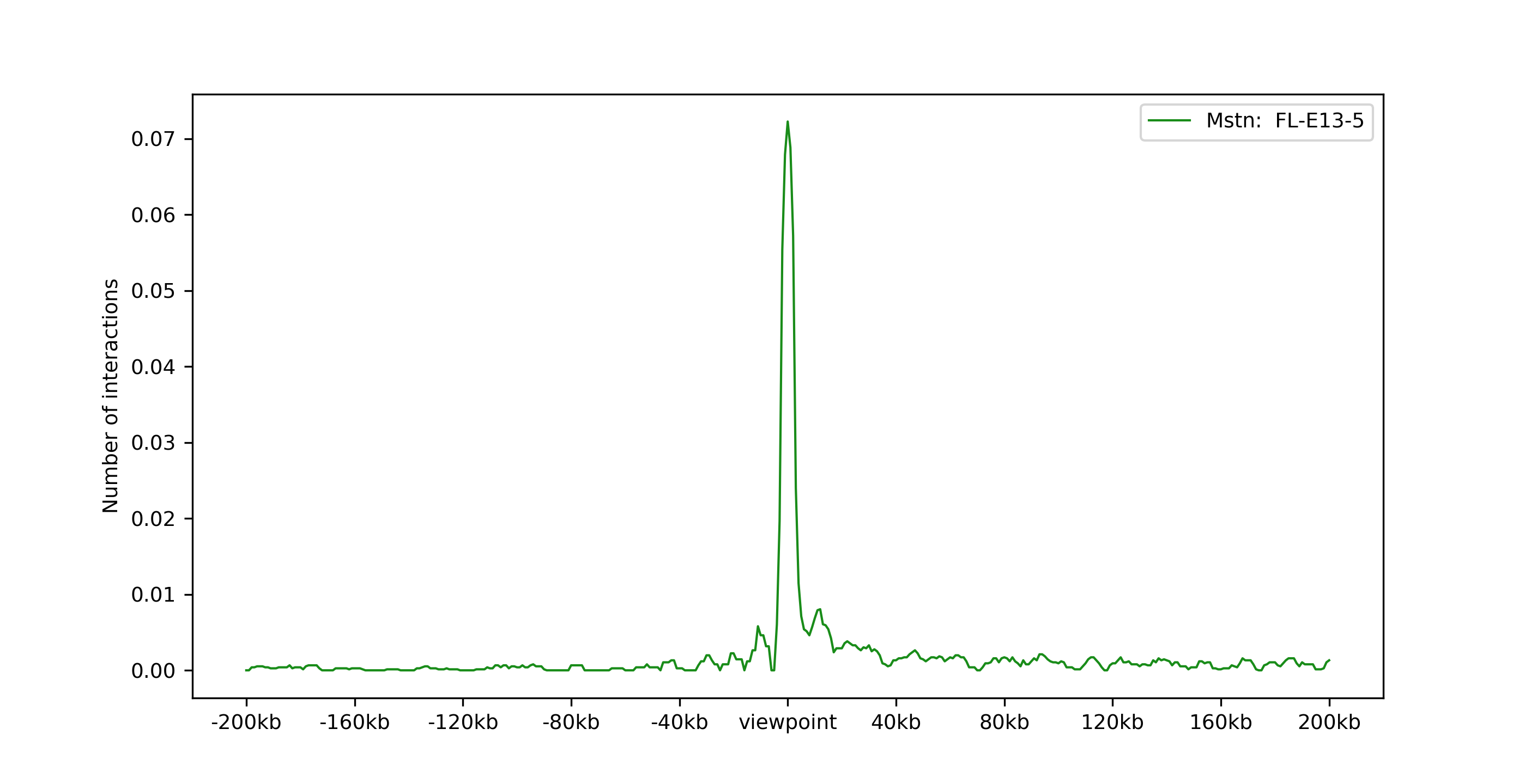
One viewpoint:
chicPlotViewpoint --interactionFile interactions.hdf5 --combinationMode oneGene --combinationName Eya1 --range 200000 200000 -o single_plot.tar.gz --outputFormat png
Two viewpoints, background, differential expression and p-values:
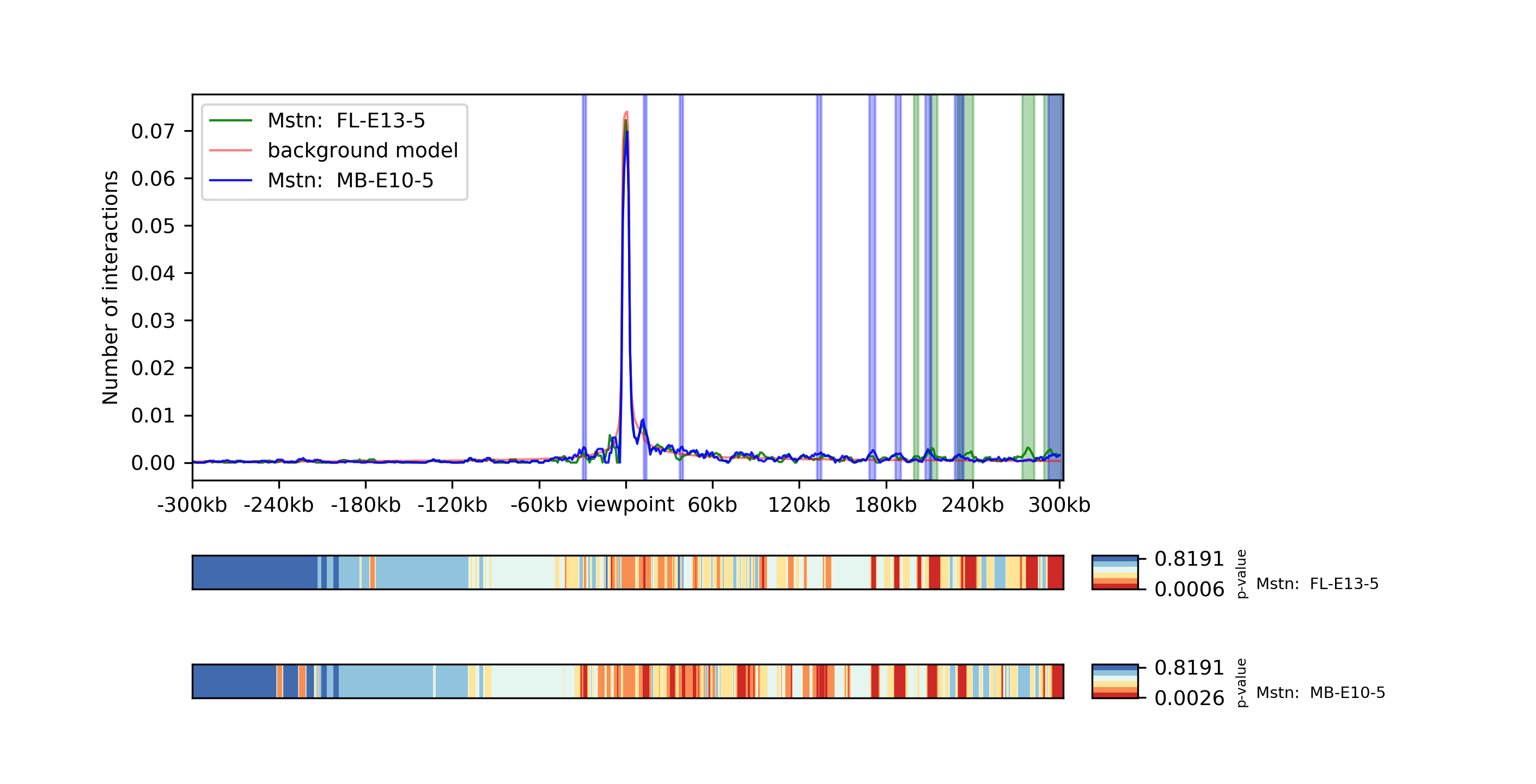
chicPlotViewpoint --interactionFile interactions.hdf5 --combinationMode dual --range 300000 300000 --pValue --differentialTestResult differential.hdf5 --backgroundModelFile background_model.txt -o differential_background_pvalue.tar.gz
This command plots two viewpoints of two different matrices of the same gene in a plot and highlights the differential regions.
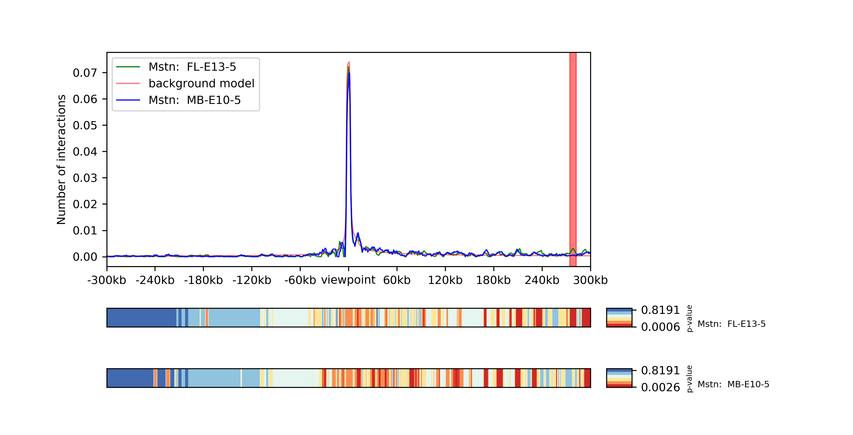
Two viewpoints, background, significant interactions and p-values:
chicPlotViewpoint --interactionFile interaction.hdf5 --combinationMode dual --range 300000 300000 --pValue --significantInteractions significant.hdf5 --plotSignificantInteractions --backgroundModelFile background_model.txt -o significant_background_pvalue.tar.gz