hicPlotTADs

Description

Plots the diagonal, and some values close to the diagonal of a Hi-C matrix. The diagonal of the matrix is plotted horizontally for a region. I will not draw the diagonal for the whole chromosome

usage: hicPlotTADs --tracks tracks.ini --region chr1:1000000-4000000 -o image.png

Required arguments

–tracks	File containing the instructions to plot the tracks. Check examples here for help to configure this .ini file: http://hicexplorer.readthedocs.io/en/latest/content/tools/hicPlotTADs.html
–region	Region to plot, the format is chr:start-end. Incompatible with –BED.
–BED	Instead of a region, a BED file containing the regions to plot can be given. If this is the case, multiple files will be created using as prefix the value of –outFileName. Incompatible with –region.

Optional arguments

–width	Figure width in centimeters. Default: 40
–height	Figure height in centimeters. If not given, the figure height is computed based on the widths of the tracks and on the depth of the Hi-C tracks, if any. Setting this this parameter can cause the Hi-C tracks to look collapsed or expanded.
–title, -t	Plot title.
–scoreName, -s
	Score name label for the heatmap legend.
–outFileName, -out
	File name to save the image, file prefix in case multiple images are stored.
–zMax	Maximum value of the score.
–vlines	Genomic cooordindates separated by space to draw vertical lines at these cooordindates. E.g. –vlines 150000 3000000 124838433
–fontSize	Font size for the labels of the plot.
–dpi	Resolution for the image in case the ouput is a raster graphics image (e.g png, jpg). Default: 72
–trackLabelFraction
	By default the space dedicated to the track labels is 0.05 of the plot width. This fraction can be changed with this parameter if needed. Default: 0.05
–version	show program’s version number and exit

Usage example

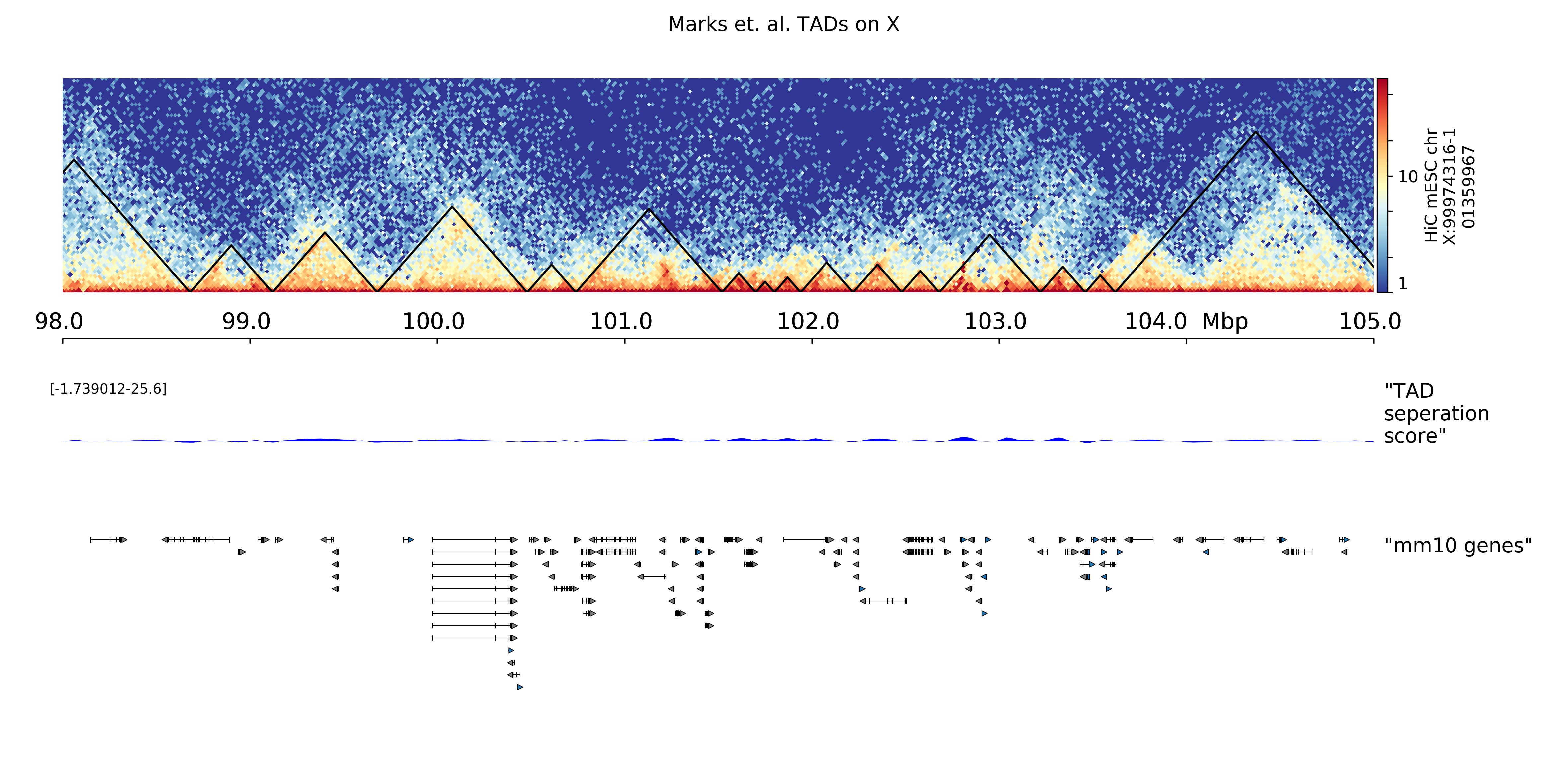
hicPlotTADs output is similar to a genome browser screen-shot that besides the usual genes, and score data (like bigwig or bedgraph files) also contains Hi-C data. The plot is composed of tracks that need to be specified in a configuration file. Once the tracks file is ready, hicPlotTADs can be used as follows:

$ hicPlotTADs --tracks tracks.ini --region chrX:99,974,316-101,359,967 \
-t 'Marks et. al. TADs on X' -o tads.pdf

Configuration file template

The following is a template for the configuration file which is based on .ini configuration files. Each track is defined by a section header (for example [hic track]), followed by parameters specific to the section as color, title, etc.

# lines that start with '#' are comment lines
# and are not interpreted by the program
# the different tracks are represented by sections in this file
# each section starts with a header of the form [hic]
# the content of the section label (in the previous example 'hic') is irrelevant for
# plotting and only used to tell the user when something goes wrong.
# There are two exceptions for this, the [x-axis] and the [spacer] sections
# that use the section label to determine the action.

[hic]
file = hic.h5
title = Hi-C
colormap = RdYlBu_r
depth = 100000
# optional arguments
min_value =2.8
max_value = 3.0
# transform options are log1p, log and -log
transform = log1p
boundaries_file = conductance_vs_hic/boundaries_all.bed
x labels = yes
type = interaction
# in case it can not be guessed by the file ending
file_type = hic_matrix
# show masked bins plots as white lines
# those bins that were not used during the correction
# the default is to extend neighboring bins to
# obtain an aesthetically pleasant output
show_masked_bins = yes

# optional, if the values in the matrix need to be scaled the
# following parameter can be used
scale factor = 1

[x-axis]
# optional
fontsize=20
# optional, options are top or bottom
where=top

# to insert a space simple add a
# section title [spacer]

[spacer]
#optional
width = 0.1

# You can also show the interactions as arcs between start and end bins.
# for this simply write the interactions in the Ginteraction format (HiCExport)
# and add the file here

[interactions]
file = Ginteractions.tsv
file_type = links
width =  10
color = black
title = HAS manual interactions
line width = 1

[bigwig]
file = file.bw
title = RNA-seq
color = black
width = 1.5
# optional values
min_value = 0
max_value = auto
# for each bin the average value is taken. The number of
# bins applies for the range being plotted. For example
# if 1Mb is plotted, then the average is computed for regions
# of 1000000/500 = 2000 bp
number of bins = 500
nans to zeros = True
# options are: line, points, fill. Default is fill
# to add the preferred line width or point size use:
# type = line:lw where lw (linewidth) is float
# similary points:ms sets the point size (markersize (ms) to the given float
type = line
# type = line:0.5
# type = points:0.5

# Default is yes, set to 'no' to turn off the visualization of
# text showing the data range (eg. 0 - 100) for the track
show data range = yes
# in case it can not be guessed by the file ending
# the file_type needs to be added
file_type = bigwig

[simple bed]
file = file.bed
title = peaks
color = read
# optional boder color. Set to none for no border color
border_color = black
width = 0.5
# optional. If not given is guessed from the file ending
file_type = bed

[genes]
# example of a genes track
# has the same options as a simple
# bed but if the type=genes is given
# the the file is interpreted as gene
# file. If the bed file contains the exon
# structure then this is plotted. Otherwise
# a region **with direction** is plotted.
file = genes.bed
title = genes
color = darkblue
width = 5
# optional
# to turn off/on printing of labels
labels = off
# options are 'genes' or 'domains'.
type = genes
# If not given is guessed from the file ending
file_type = bed
# optional: font size can be given if default are not good
fontsize = 10

[chrom states]
# this is a case of a bed file that is plotted 'collapsed'
# useful to plot chromatin states if the bed file contains
# the color to plot
file = chromatinStates.bed
title = chromatin states
# color is replaced by the color in the bed file
# in this case
color = black
# optional boder color. Set to none for no border color
border_color = black
# default behaviour when plotting intervals from a
# bed file is to 'expand' them such that they
# do not overlap. The display = collapsed
# directive overlaps the intervals.
display = collapsed
width = 0.3

[bedgraph]
file = file.bg
title = bedgraph track
color = green
width = 0.2
# optional. Default is yes, set to no to turn off the visualization of data range
show data range = yes
# optional, otherwise guessed from file ending
file_type = bedgraph


[bedgraph matrix]
# a bedgraph matrix file is like a bedgraph, except that per bin there
# are more than one value separated by tab: E.g.
# chrX       18279   40131   0.399113        0.364118        0.320857        0.274307
# chrX       40132   54262   0.479340        0.425471        0.366541        0.324736
# bedgraph matrices are produced by hicFindTADs
file = spectra_conductance.bm
title = conductance spectra
width = 1.5
orientation = inverted
min_value = 0.10
max_value = 0.70
# if type is set as lines, then the TAD score lines are drawn instead
# of the matrix
# set to lines if a heatmap representing the matrix
# is not wanted
type = lines
file_type = bedgraph_matrix

[vlines]
# vertical dotted lines from the top to the bottom of the figure
# can be drawn. For this a bed file is required
# but only the first two columns (chromosome name and start
# are used.
# vlines can also be given at the command line as a list
# of genomic positions. However, sometimes to give a file
# is more convenient in case many lines want to be plotted.
file = regions.bed
type = vlines